The gentle rocking of a boat can be a soothing lullaby. But when that gentle rock turns into a violent, unpredictable roll, it’s anything but. For centuries, naval architects have worked to counteract this roll, especially when a ship is at its most vulnerable—at anchor, with no forward speed to aid stability. Traditional solutions work well, but what if we could make them smarter? What if a ship’s control system could learn, adapt, and react to the waves with the intuition of a seasoned sailor?
This is the story of how we took on that challenge. We’re going to take a deep dive into the world of artificial intelligence to show you how we trained an AI agent, from scratch, to master the complex art of ship roll stabilization. Forget everything you know about manually tuned controllers; we’re entering the era of data-driven, self-learning systems.
Building a Digital Ocean
You don’t teach an AI to swim by throwing it into the ocean. You build it a world-class digital swimming pool first. It’s simply not feasible (or safe!) to train a reinforcement learning (RL) agent on a real multi-million dollar yacht. We needed a robust, high-fidelity simulation environment where our agent could experiment, fail, and learn millions of times over without consequence.
We developed a custom environment, compatible with the industry-standard OpenAI Gym, that accurately emulates the roll dynamics of a ship. This became the playground for our RL agent. The interaction is a continuous loop—a dialogue between the “Agent” (the AI brain) and the “Environment” (the simulated ship).
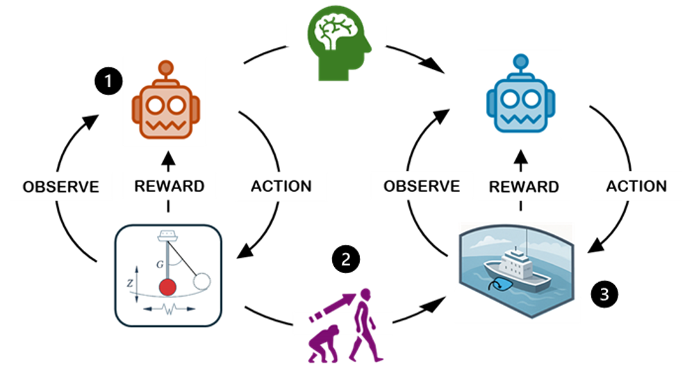 Figure 1: The fundamental agent-environment feedback loop of reinforcement learning.
At every time step (in our case, every 0.25 seconds), this dialogue unfolds:
- Observation: The Environment tells the Agent what’s happening. This isn’t just a single number; it’s a vector of crucial data:
\(o_t = [\phi, \dot{\phi}, \ddot{\delta}, \delta_{act}]^T\)
- \(\phi\): The current roll angle of the ship.
- \(\dot{\phi}\): The current roll rate (how fast it’s rolling).
- \(\ddot{\delta}\): The fin’s angular acceleration.
- \(\delta_{act}\): The actual, current angle of the stabilization fin.
- Action (\(a_t\)): Based on this observation, the Agent makes a decision: what should the new target angle for the fins be?
- Reward (\(r_t\)): The Environment responds with a scalar “reward” signal. This is the critical feedback that guides the entire learning process.
To make the challenge realistic, we imposed physical limits, just as a real fin system would have.
Table 1: Observation and action limits used in the RL workflow.
| Symbol |
Physical meaning |
Range (deg) |
| \(\phi\) |
Roll angle |
[-60, +60] |
| \(\dot{\phi}\) |
Roll rate (deg/s) |
[-360, +360] |
| \(\ddot{\delta}\) |
Fin angular accel. (\(deg/s^2\)) |
[-60, +60] |
| \(\delta_{act}\) |
Actual fin angle |
[-30, +30] |
| \(a_t\) |
Commanded fin angle |
[-30, +30] |
The Brains of the Operation
With our digital ocean ready, we needed an AI “brain” to navigate it. We chose a powerful, state-of-the-art RL algorithm called Soft Actor-Critic (SAC). While other methods like Model Predictive Control (MPC) are powerful, they require an accurate model of the system dynamics. We chose SAC for its model-free nature, allowing it to learn directly from interaction in our complex, nonlinear environment.
The SAC Algorithm in Detail
The “soft” in Soft Actor-Critic comes from its core objective, which is based on the maximum entropy reinforcement learning framework. Unlike traditional RL algorithms that solely aim to maximize the cumulative reward, SAC aims to maximize a combination of the expected reward and the entropy of the policy.
The optimization objective is:
\[\pi^* = \arg\max_\pi \sum_t \mathbb{E}_{(\mathbf{o}_t, \mathbf{a}_t) \sim \pi} \left[ r(\mathbf{o}_t, \mathbf{a}_t) + \alpha \mathcal{H}(\pi(\cdot|\mathbf{o}_t)) \right]\]
Let’s break this down:
- \(\pi^*\): This represents the optimal policy we are trying to find.
- \(\mathbb{E}_{...}[r(o_t, a_t)]\): This is the standard RL objective—the expected cumulative reward ((r)) over time.
- \(α H(π(\cdot \| o_t))\): This is the entropy bonus, the secret sauce of SAC.
- \(H(π(\cdot \| o_t))\) is the Shannon entropy of the policy \(\pi\). Entropy is a measure of randomness. By maximizing entropy, the agent is encouraged to explore and avoid collapsing into a deterministic, and potentially sub-optimal, strategy too early.
- \(α\) is the temperature parameter, which controls the importance of the entropy term versus the reward. A higher \(α\) means more exploration. In modern SAC implementations, this is a tunable parameter that is automatically adjusted to maintain a target entropy.
Implementation Details
For reproducibility, the key hyperparameters and training details are provided below. The agent was trained for approximately 500,000 environment steps, which converged in a matter of hours on a standard desktop GPU.
Table 4: Key training hyperparameters.
| Parameter |
Value |
| RL Algorithm |
Soft Actor-Critic (SAC) |
| Learning Rate |
3 × 10⁻⁴ |
| Discount Factor (\(\gamma\)) |
0.99 |
| Replay Buffer Size |
5 × 10⁵ |
| Batch Size |
512 |
| Target Update (\(\tau\)) |
0.005 |
| Optimizer |
Adam |
| Network Architecture |
2x128 Hidden Layers (tanh) |
A Curriculum for a Digital Sailor
Having a brain and a playground isn’t enough. You need a curriculum. For an RL agent, the curriculum is defined by the reward function and the training regimen.
The Reward: Defining ‘Good’
The reward function is how we communicate our goal to the agent. Our objective is to achieve stable and efficient roll damping. We translated this into a concrete mathematical formula. The reward \(R_t\) at any time step \(t\) is:
\[R_t = -w_\phi\,\phi_t^2 - w_{\dot\phi}\,\dot\phi_t^2\]
This function explicitly penalizes two things: the squared residual roll angle (\(\phi_t^2\)) and the squared roll rate (\(\dot\phi_t^2\)). By penalizing the square of the values, we disproportionately punish larger deviations, strongly encouraging the agent to keep the ship stable. The weights \(w_{\phi}\) and \(w_{\dot{\phi}}\) allow us to balance the importance of these two objectives.
The Training Regimen: Domain Randomization
We don’t want an agent that is a one-trick pony. To create a robust, seasoned sailor, we used Domain Randomization. Instead of training on a single sea state, we subjected the agent to a wide and constantly changing variety of conditions at the start of every training episode.
Table 2: Domain randomization envelope for sea-state parameters.
| Parameter |
Min/Max or Value |
| \(H_s\) (significant height) |
[0.5 m, 2.0 m] |
| \(T_p\) (peak period) |
[8 s, 12 s] |
| Heading (relative) |
Fixed beam seas (90°) |
| Wave seed |
[0, 10⁶] |
This process forces the agent to learn a generalized policy that is effective across a whole family of sea states, making it incredibly resilient.
Graduation Day
The Baseline: A Conventional Controller
Before looking at our RL agent’s results, it’s important to understand the baseline. A conventional approach to this problem is a Saturated Proportional-Derivative (SPD) controller. It’s a reliable, classic control strategy that adjusts the fins based on the current roll angle (the Proportional term) and the roll rate (the Derivative term). The “Saturated” part means its commands are capped at the physical limits of the fin hardware. While effective, it must be manually tuned for a specific set of conditions.
The Training Results
After millions of simulation steps, our agent was ready. The training curves below show a clear story: the agent steadily improved its performance, reducing the ship’s roll and maximizing its reward.
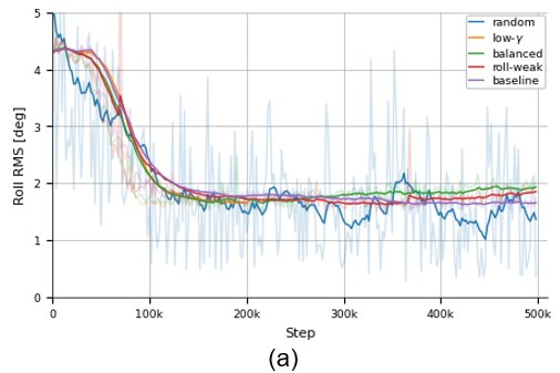
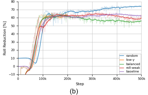
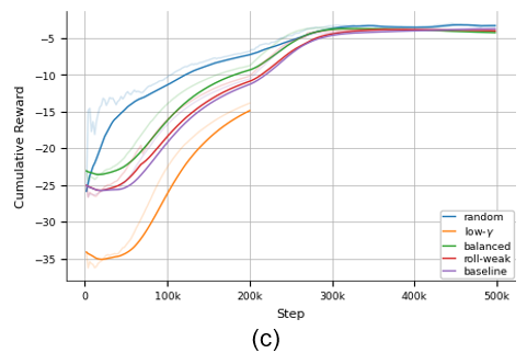 Figure 2: Training process key indicators showing: (a) Roll RMS decreases, (b) Roll Reduction increases, and (c) Cumulative Reward.
Model Evaluation
The time-series plots below give a dramatic visual of the agent’s success. Both the specialist agent (trained on a single wave pattern) and our robust generalist significantly suppress the roll compared to the uncontrolled “passive” state.
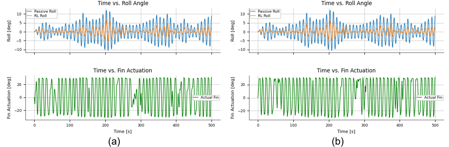 Figure 3: Time-trace comparison for (a) a single-wave agent and (b) our random-domain agent. The Orange line (RL Roll) shows the reduction in motion compared to the uncontrolled Blue linee (Passive Roll).
A key metric in RL is “sample efficiency”—how much data is needed to learn? The graph below plots performance against training time.
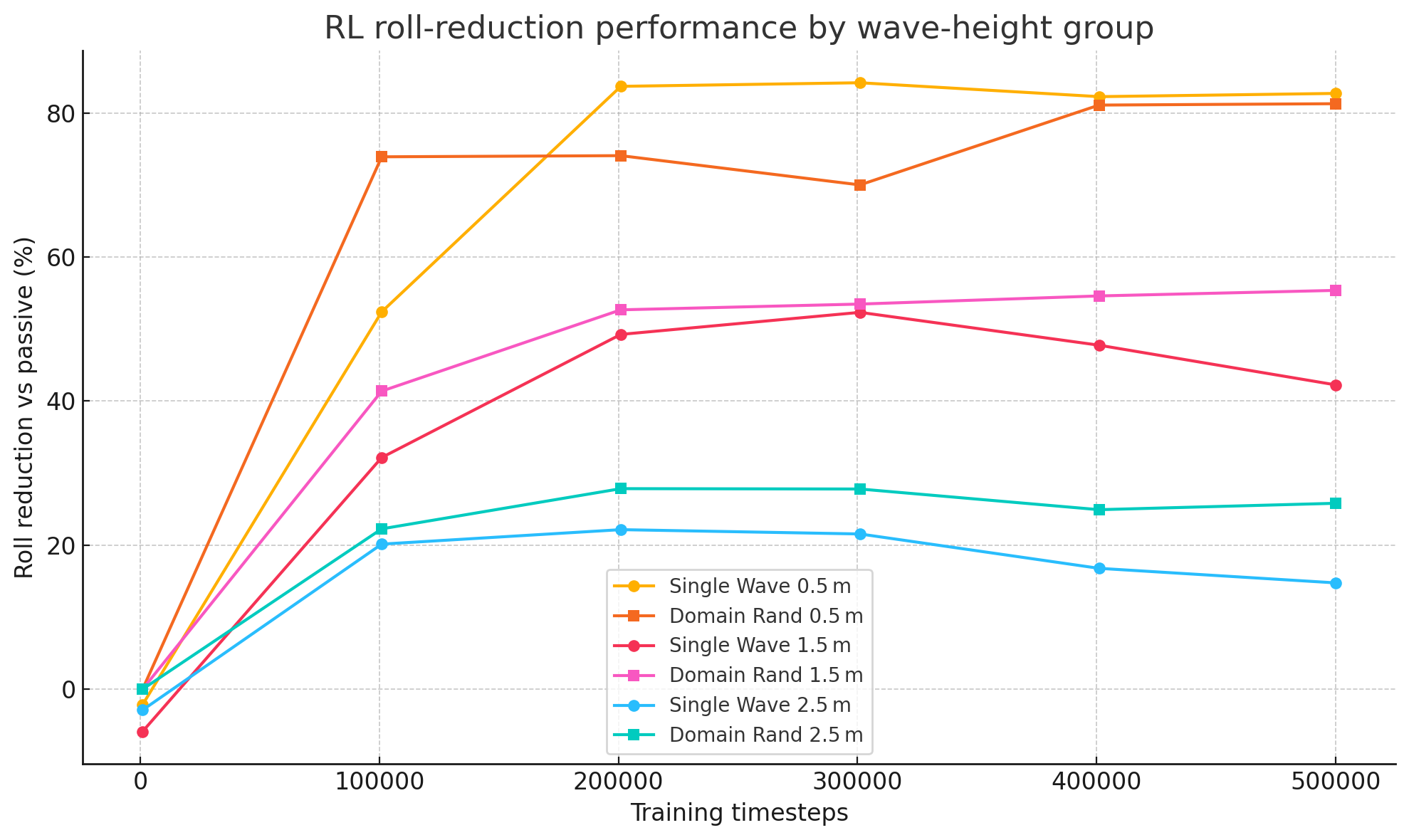 Figure 4: Sample efficiency showing roll reduction vs. training data for different sea states. The RL agents demonstrate a clear learning trajectory as they accumulate experience.
The final numbers speak for themselves. In the most challenging sea states, the robust, multi-wave RL agent even outperformed the specialist agent, proving the power of domain randomization.
Table 3: Final roll reduction percentage.
| Wave height |
RL single wave |
RL multiple waves |
| 0.5 m |
84% |
81% |
| 1.5 m |
52% |
55% |
| 2.5 m |
22% |
28% |
The Future is Adaptive
This project proved that Reinforcement Learning has immense potential. While conventional controllers still hold an edge in tuning speed, the path forward is clear.
Our next steps are to push the boundaries even further:
- Give the Agent a Memory: Implement advanced network architectures like LSTMs that can recognize long-term wave patterns.
- Expand its Senses: Feed the agent more data, like heave and pitch motion, so it can anticipate coupled motions.
- The Hybrid Approach: The ultimate goal may not be to replace classical controllers, but to augment them. Imagine a system where a proven controller handles the basics, and an RL agent learns to provide small, intelligent corrections on top. This offers the best of both worlds: the reliability of classical control and the adaptive power of AI.
We are just scratching the surface of what is possible. The future of ship control is not just automated; it’s adaptive, intelligent, and continuously learning.